In this section we introduce the basics of parsing theory. A deeper treatment would be more appropriate as part of a compilers course. We will discuss some preliminary concepts, then look into top-down parsing (LL-parsers) and conclude with bottom-up parsing (LR-parsers).
Resources:
A parser takes as input a CFG and an input string. The parser must then produce a valid parse tree for this string, ideally a unique parse tree, or else say why such a parse tree cannot exist. In order to do this, the parser must look at the beginning of an input string and determine what production rules it should consider when many rules are applicable. As a preparation for this, we will discuss first and follow sets, which help the parser decide.
Whatever parser approach we take, at some point we are presented with the problem of deciding which production rule to consider where many are applicable. A helpful step in the process is knowing what terminals can appear at the start of a string derived from a given nonterminal, and similarly knowing what terminals can follow a string derived from a given nonterminal. These sets have names:
For a symbol \(X\) in a CFG:
- The first set of \(X\), written \(\textrm{FIRST}(X)\), is the set of all terminals (including \(\epsilon\)) that can appear as the first character in a string derived from \(X\). For the case of \(\epsilon\), we only include it if the symbol \(X\) can derive the empty string.
- The follow set of \(X\), written \(\textrm{FOLLOW}(X)\), is the set of all terminals (not including \(\epsilon\) but including the end-of-input marker \(\$\)) that can immediately follow \(X\) in a sentential form. A sentential form is any sequence of terminals and nonterminals that can be derived from the start symbol. So sentential forms are valid intermediate results on the way to deriving a string in the language.
The first sets are computed via a “closure” process, described by the following rules:
Construction of first sets
- If \(X\) is a terminal, then \(\textrm{FIRST}(X) = \{X\}\) contains only that terminal.
- If \(X\to\epsilon\) is a production rule, then \(\epsilon\in\textrm{FIRST}(X)\).
- If we have a production \(X\to Y_1Y_2\cdots Y_k\), then:
- \(\textrm{FIRST}(Y_1)\subset\textrm{FIRST}(X)\)
- If \(\epsilon\in \textrm{FIRST}(Y_1)\) then \(\textrm{FIRST}(Y_2)\subset\textrm{FIRST}(X)\).
- If \(\epsilon\in \textrm{FIRST}(Y_1)\) and \(\epsilon\in \textrm{FIRST}(Y_2)\) then \(\textrm{FIRST}(Y_3)\subset\textrm{FIRST}(X)\).
- More generally, if \(\epsilon\) is in the first set of each of the symbols \(Y_1,Y_2,\cdots,Y_{i-1}\), then \(\textrm{FIRST}(Y_i)\subset\textrm{FIRST}(X)\).
- If \(\epsilon\) is in the first set of all the symbols \(Y_1,Y_2,\cdots,Y_k\), then \(\epsilon\in\textrm{FIRST}(X)\).
We follow these rules repeatedly over all the production rules of the grammar until we obtain nothing new.
We will illustrate this in the example of simple algebraic expressions. The alphabet is \(\Sigma=\{x, +, *, (, )\}\), where \(x\) represents the location of a number (the actual numerical value is usually communicated via other means).
S -> E
E -> E + T | T
T -> T * F | F
F -> x | ( E )
To find the first sets, we start by considering the terminals, and setting their first sets.
Symbol        First Set
------------  ----------------
x             x
+             +
*             *
(             (
)             )
S
E
T
F
For simplicity we will only worry about the nonterminals from now on.
We start with the rules for S. The only production we have is S->E, therefore the first set of E must be contained in the first set of S. Since we don’t have any elements in the first set of E yet, this gives us no elements for the first set of S.
Similarly, the rules for \(E\) and \(T\) won’t give us any first set elements yet.
We continue with the rules for \(F\). Looking at its two productions, we can determine that \(x\) and the open parenthesis must be in the first set of \(F\).
We next revisit the rules for \(T\), now that we know something about \(F\). The first rule has \(T\) on its left-hand side, telling us that the first set of \(T\) will contain everything in the first set of \(T\), not very helpful. But the second rule tells us that the first set of \(T\) will contain anything in the first set of \(F\), which so far is the elements \(x\) and open parenthesis.
The same logic would apply to \(E\). So in this case all 3 variables have the same first set so far, namely the set {x, (}. It makes sense, since these are the only two valid starts of an expression. So at this point the first sets are as follows:
Symbol            First Set
--------          -----------
S
E                 x, (
T                 x, (
F                 x, (
If we now make a another pass through the rules, we discover that S must have two first set elements, since the first set of E acquired those two elements.
If we try to look at any of the rules again, we don’t get any new entries. Sometimes there is more work involved. In our case, the final list of first sets is:
Symbol            First Set
--------          -----------
S                 x, (
E                 x, (
T                 x, (
F                 x, (
Now we will discuss follow sets, which are built based on similar ideas.
Construction of follow sets
- \(\$\in\textrm{FOLLOW(S)}\).
- If there is a production rule \(A\to \alpha B \beta\), then \(\textrm{FIRST}(\beta)\subset\textrm{FOLLOW}(B)\).
- If there is a production rule \(A\to \alpha B\) or a rule \(A\to \alpha B \beta\), where \(\epsilon\in\textrm{FIRST}(\beta)\), then \(\textrm{FOLLOW}(A)\subset\textrm{FOLLOW}(B)\). This is because if we can reduce everything following \(B\) to \(\epsilon\), then the production for \(A\) may end in \(B\), so anything that can follow an \(A\) can also follow a \(B\).
Let us illustrate this process in our example. We start with the rule for \(S\): \(S \to E\). The third rule above tells us to add to the follow set of \(E\) anything in the follow set of \(S\), namely \(\$\).
Next we look at the rules for \(E\). It seems they tell us that everything in the follow set of \(E\) must be in the follow set of \(T\). And similarly from the rules for \(T\) we find that everything in the follow set of \(T\) must be in the follow set of \(F\). So we add the end symbol to the follow sets for \(E\), \(T\) and \(F\).
Now we come to the rules for \(F\). One says that \(F\to x\), and that has no useful information for us. The other says \(F\to (E)\), which tells us by the second follow rule above that the closing parenthesis is in the follow set of \(E\) (and hence also in the follow sets of \(T\) and \(F\) by our previous paragraph). This gives us the final table:
Symbol            First Set               Follow Set
--------          -----------             -----------
S                 x, (                    $
E                 x, (                    $, )
T                 x, (                    $, )
F                 x, (                    $, )
We have not yet fully accounted for the rules E->E+T and T->T*F. It is clear that E may be followed by a plus, and T may be followed by a star. These transfer to the other sets as appropriate.
Symbol            First Set               Follow Set
--------          -----------             -----------
S                 x, (                    $
E                 x, (                    $, +, )
T                 x, (                    $, +, *, )
F                 x, (                    $, +, *, )
And this is our final table! It tells us for example that a single factor (\(F\)) may be followed by:
As a second example, let us consider implementing a grammar for “Polish notation”. Polish notation places the operators in front of the two operands. For example instead of writing: (5 + 6) * 7 it would write * + 5 6 7. On the other hand 5 + 6 * 7 would have been + 5 * 6 7. The awesome thing about Polish notation is that it is unambiguous, no parentheses are needed (though perhaps we would feel more comfortable writing the last expression for instance as (+ 5 (* 6 7)), which is the LISP/Racket programming language style). Let us see how the grammar would look (we use different symbols to visually distinguish it from the earlier work, using P for “Polish expression”, and \(y\) for the variable representing numbers):
S -> P
P -> + P P | * P P | y
Hm, exciting! As an example of a derivation in this language, consider the building of the string: * + y y y
S => P => * P P => * + P P P => * + y P P => * + y y P => * + y y yLet us try to compute the first and follow sets in this example. The language alphabet is { y,+,* }, so they are each their own first sets.
P -> y tells us that y is in the first set of P.P -> + P P and P -> * P P tell us that +,* are in the first set of P.S -> P tells us that everything in the first set of P is in the first set of S.So we end up with:
Symbol            First Set
--------          -----------
S                 y, +, *
P                 y, +, *
Okay perhaps it was not all that exciting at the end of the day.
Now let us look at follow sets:
$ is in the follow set of \(S\).P -> + P P says, looking at the two Ps at the end and thinking of this rule as a \(A\to \alpha P \beta\), that anything in the first set of P (the second of those two Ps) must be in the follow set of P (the first of those two Ps). Same for the other rule. So \(\textrm{FIRST}(P)\subset\textrm{FOLLOW}(P)\).S -> P, anything in the follow set of S is in the follow set of P.We can visualize these rules as follows, by considering the various ways we can write our production rules as A -> alpha B beta or A -> alpha B:
A   alpha  B      beta  Conclusion
--- -----  ---    ----- -----------------------
S          P            FOL(S) subset of FOL(P)
P   + P    P            FOL(P) subset of FOL(P)
P   +      P      P     FIR(P) subset of FOL(P)
P   * P    P            FOL(P) subset of FOL(P)
P   *      P      P     FIR(P) subset of FOL(P)
So we end up with:
Symbol            First Set               Follow Set
--------          -----------             -----------
S                 y, +, *                 $
P y, +, * y, +, *, $The idea of LL-parsers is simple, and closely follows the pushdown automaton we built from a grammar. In essence:
This is considered a top-down approach: As we imagine the resulting parse tree, we start from the top and decide what rule to expand it to, then proceed to do the same for each child node. So we build the parse tree from the top and move towards the bottom.
Of course you will now wonder: How do we choose which production rule to use at any given time? If we choose the wrong one we will get stuck. There are two approaches:
P which rule to follow next, but peeking at the next input symbol helps us out: If it is + then we use the rule P -> + P P, if it is * we use P -> * P P and if it is y we use P -> y. The fact that the first set of P consists of only these three terminals tells us that this is what we expect to see next in our input; anything else would be an error (e.g. end-of-input symbol indicating an error like + 2 without a second term).These parsers are called LL(k) parsers, where \(k\) indicates the number of lookahead symbols required, LL(0) being the case of no lookahead at all and LL(1) being the case we just examined for the Polish notation. A grammar is called LL(k) if it gives rise to an unambiguous (deterministic) LL(k) parser. A language is LL(k) if it has a grammar that is LL(k).
The first L in “LL” refers to the fact that these parsers process their input from left to right, while the second refers to the fact that they trace a leftmost derivation of the parse tree. These parsers are also often described as predictive, since they need at any given time to “predict” which rule would be the correct one to apply. This contrasts them with the LR parsers that we will discuss shortly.
The information needed for implementing an LL(k) parser is typically stored in a “parse table”, whose rows correspond to different nonterminal symbols and whose columns correspond to the various possible lookaheads (so for a large \(k\) we could have a very large number of columns). The entry in the table describes the rewrite rule. For LL(1) parse tables, the construction essentially follows the process for finding first sets. Every new element we add to a first set gives rise to an entry in the table, based on the rewrite rule used to deduce it. If we find that we are “rediscovering” an element, that means there is a conflict with two rules matching the same “next symbol”. The parser would not know which one to pick.
For our Polish notation example, the LL(1) parse table would look as follows:
Nonterminal     y        +          *           $ (end of string)
-----------     ---      ------     -------     -------
S               P        P          P           error
P               y        + P P      * P P       error
The main principle here is this:
- The lookahead symbol must be in the first set of the variable we are trying to match.
- The production rule that helped us learn that this symbol is in this first set is the rule we want to apply.
- If we can learn this fact from two different production rules, we have a conflict.
And here are the steps that the LL-parser would follow:
Input        Stack      What happened
----------   ---------  ---------------
+*yyy        $S         start
+*yyy        $P         S -> P
+*yyy        $PP+       P -> +PP
*yyy         $PP        read +
*yyy         $PPP*      P -> *PP
yyy          $PPP       read *
yyy          $PPy       P -> y
yy           $PP        read y
yy           $Py        P -> y
y            $P         read y
y            $y         P -> y
eps          $          read y
The steps above follow a left-most derivation, namely:
S -> P -> +PP -> +*PPP -> +*yPP -> +*yyP -> +*yyyBefore moving on, let us revisit the arithmetic expressions example we started with. We are already seeing a case where LL(k) parsers are not sufficient. For simplicity, consider the language:
E -> T         (1)
E -> E + T     (2)
T -> v         (3)
T -> ( E )     (4)
We will now consider how LL(1) parsing of this language will go, based on a computation of first sets. The rules tell us the following:
Rule          Conclusion
-----------   ----------------------------
E -> T        FIRST(T) subset of FIRST(E)
E -> E + T    FIRST(E) subset of FIRST(E)
T -> v        v in FIRST(T)
T -> ( E )    ( in FIRST(T)
The second statement above might sound trivial, but is in fact the problem. Here is how the LL(1) parse table would look:
Variable     v      +      (       )
---------    -----  -----  ------  ----
E            (1,2)         (1,2)
T            (3)           (4)
The problem is the following: We first find out that x can be in the first set of E because of the E->T rule. But then we learn it again because x is in E and we have the rule E->E+T. This means that when we encounter an x in our attempt to match an E, we don’t know if we should apply rule 1 or rule 2, they both are possibilities. In order to answer that question, we may need to look deeper into our string, to see if there is a plus following our x or not. (In the case of the parenthesis, we might have to search ahead for quite a while until we find the closing parenthesis).
Essentially, the problem is that we have no way of choosing which of the rules \(E\to E+T\) and \(E\to T\) is the correct one to apply next, namely whether the expression is just one term or the sum of two terms. We would need to somehow be able to look far enough ahead into the expression to see if that “plus” is there or not. But that expression could be arbitrarily long, containing millions of parentheses on the way. No amount of lookahead can help us here.
In general this is a difficulty that LL(k) parsers have with what are known as left-recursive grammars, namely grammars that contain a production rule for a nonterminal, whose right-hand side has that same nonterminal as its first element (like the expression E->E+T above). These grammars almost invariably force the LL parser to commit too soon, before it has enough information to make a decision.
Luckily left-recursive grammars can be rewritten to not be left-recursive. It is not enough to simply write it instead as \(E\to T + E\), because that changes the associativity semantics. It may not matter because addition is associative, but in other cases it would matter a lot. Instead, we can rewrite such a grammar as follows:
E -> T X     (1)
X -> eps     (2)
X -> + T X   (3)
T -> v       (4)
T -> ( E )   (5)
Take a moment to make sure you understand that this did not change the associativity. In particular:
Exercise: work out the parse tree for the string v+v in this language. You should come up with the following derivation:
   1       4       3           4           2
E ==> T X ==> v X ==> v + T X ==> v + v X ==> v + v
The big difference in this language is that we have a production rule for X that produces an empty string. The question we need to answer is: When should this rule be applied? We cannot use the first set of X, because this rule does not bring anything to the first set, in fact it is not going to consume any input. But we can instead look at the follow set of X: If the lookahead symbol is in the follow set of X, then it is worth it to consider the epsilon-production for X, as this symbol may follow X and hence we may have the X appear at this position.
Let us consider therefore the above rules and what they teach us about follow sets:
A      alpha  B      beta  Conclusion
---    -----  ---    ----- ------------------------
E             T      X     FIR(X) subset of FOL(T)
E             T      X     FOL(E) subset of FOL(T)
E      T      X            FOL(E) subset of FOL(X)
X      +      T      X     FIR(X) subset of FOL(T)
X      +      T      X     FOL(X) subset of FOL(T)
X      + T    X            FOL(X) subset of FOL(X)
T      (      E      )     ) in FOL(E)
And of course we should also consider what they teach us about first sets:
Rule         Conclusion
-----------  ----------------------------
E -> T X     FIRST(T) subset of FIRST(E)
X -> eps
X -> + T X   + in FIRST(X)
T -> v       v in FIRST(T)
T -> ( E )   ( in FIRST(T)
Now we build our LL(1) table. We start by filling in the conclusions from first sets.
Variable     v       +       (        )      $
---------    ------- ------- -------  ------ -------
E            E->TX           E->TX
X                    X->+TX
T            T->v            T->(E)
Now we fill in entries based on follow set symbols, for the variable X that has epsilon production rules. Recall that the end of input symbol is always in the follow set of the start variable, E in our case:
Variable     v       +       (        )       $
---------    ------- ------- -------  ------- -------
E            E->TX           E->TX
X                    X->+TX           X->eps  X->eps
T            T->v            T->(E)
If, in the process of parsing string s, we hit a ‘blank spot’ in the parsing table (a place in the table with no entry), then that string is ungrammatical; it cannot be parsed in this case because it is not in the language of the grammar, therefore the parser ends up getting stuck. This is usually called a parse error.
For completeness, what follows is the same transformation for the bigger grammar with terms and factors:
E -> T | E + T
T -> F | T * F
F -> x | ( E )
And the transformed grammar would look as follows:
E -> T X
X -> eps | + T X
T -> F Y
Y -> eps | * F Y
F -> x | ( E )Exercise: Compute the first and follow sets for this grammar. You should end up with the following table:
Symbol            First Set               Follow Set
--------          -----------             -----------
S                 x, (                    $
E                 x, (                    ), $
X                 eps, +                  ), $
T                 x, (                    ), +, $
Y                 eps, *                  ), +, $
F                 x, (                    ), +, *, $
Let us now attempt to build an LL(1) table for this grammar. We have one new interesting case to consider, because of epsilon production rules like \(A\to\epsilon\). We apply such a rule if the lookahead symbol could follow \(A\). Omitted entries indicate error.
Symbol      x       +       *        (       )      $ (end of string)
------     ---     ---     ---      ---     ---    ---
S           E       -       -        E       -      -
E          T X      -       -       T X      -      -
X           -     + T X     -        -      eps    eps
T          F Y      -       -       F Y      -      -
Y           -      eps    * F Y      -      eps    eps
F           x       -       -       (E)      -      -
As long as we do not encounter any conflicts (e.g. two rules both claiming the same spot), we have an LL(1) parser.
Exercise Consider the palindrome grammar we discussed earlier.
Exercise Consider the language \(L=\{x^n\mid n\geq 0\}\cup\{x^ny^n\mid n\geq 0\}\).
This language is not LL(k) for any \(k\). Try to explain why (it is not just that your grammar is not LL(k), it’s that there cannot be a LL(k) grammar for this language).
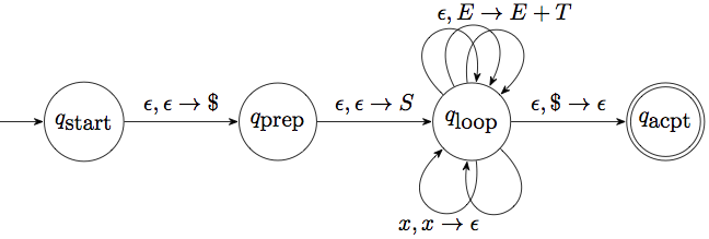
The LL parsers we just described essentially carry out the pushdown automaton we built from a CFG back when we were trying to establish the correspondence between PDAs and CFGs, which looked something like this:
So after we place the empty-stack symbol and the start symbol onto the stack, we perform a series of steps that are all either removing a terminal from the stack if it matches the input, or replacing the nonterminal at the top of the stack with a production rule for it.
There is another PDA that can serve a similar purpose, but it works in a somewhat “dual” way: It can push terminals it encounters on the input onto the stack (a step called shift), and if it finds the right-hand side of a production rule at the top spots of the stack then it can replace it with the nonterminal on the left-hand side of the rule ( a step called reduce). Graphically this would look something like this:
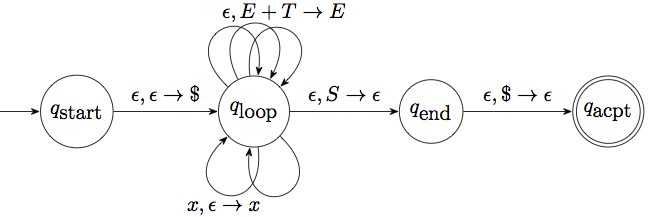
This turns out to correspond to a bottom-up approach of building the parse tree. We first build the child nodes of a production rule, then replace them with the parent node. This results in a “rightmost” derivation, hence the “R” in “LR”.
The key observation (which will become clear later) is this:
At any given time, the stack of an LR parser contains part of the right-hand side of a production rule. These possible states of the stack can be coded into a DFA.
As an example, let us consider how the stack would track the expression + * y y y from the Polish notation example, before we build more of the theory:
Input          Stack        What happened
-----          -----        -------------
+*yyy          $            start
*yyy           $+           push +
yyy            $+*          push *
yy             $+*y         push y
yy             $+*P         P -> y
y              $+*Py        push y
y              $+*PP        P -> y
y              $+P          P -> * P P
eps            $+Py         push y
eps            $+PP         P -> y
eps            $P           P -> + P P
eps            $S           S -> P
eps            $            pop S and advance to end/accept
You will notice that we have violated one of the rules of the stack: In order to see that we have a * P P in the stack, we actually have to look 3 places deep. We will discuss later how to get around this problem.
We need a way to discuss in general the idea that “we have seen a part of the right-hand side of a rule”. For that we need a new definition:
An item is a production rule with a specific marker somewhere amongst the right-hand side symbols. The marker is typically denoted by a dot. For instance the production rule
P->+PPgives rise to 4 items:P->.+PP,P->+.PP,P->+P.P,P->+PP..An “item” suggests that we are working towards matching this rule, and we have so far matched the symbols on the left of the dot. These symbols are waiting comfortably at the top of the stack for the rule to be completed.
So items effectively represent “stages”. An item with the marker all the way to the left is said to be in initial form, one with the marker all the way to the right is said to be in terminal form. Items in terminal form are ready to be replaced by the left-hand side of the production rule.
As an example, let us revisit the polish notation example we have been working on. We can imagine that we are trying to parse the string * y y. Then we can look at the following sequence of items:
Item            Input           What's going on
------------    ---------       -------------------------------------------
S -> .P         * y y           Starting to parse, looking for a P
P -> .* P P     * y y           To get a P, looking for a star
* . P P         y y             Read the star, looking for a P
P -> .y         y y             To get a P, looking for a y
P -> y.         y               We read the y
P -> * P . P    y               With that y we have succesfully read a P. Look for next P
P -> .y         y               To get a P, looking for a y
P -> y.                         Read y from input
P -> * P P .                    With that y we have formed a P.
S -> P.                         We have successfully read a *PP, convert it to a P
                                Done
What happens in the above example is that certain items are “related” to each other. For example the item S -> .P is closely related to the item P -> .* P P, because the first item expresses our desire to find a P, and the second item offers us a start at finding a P. This leads us naturally to the following definition of “item sets”:
An item set is a set of items that has had a “closure” operation performed on it as follows: For any of the items in the set, if there is a nonterminal appearing immediately to the right of the marker, then we add items in initial form for all production rules for that nonterminal.
For example, here are some item sets we might have in the polish notation example:
Set 1: S -> .P      P -> .y      P -> .* P P       P -> .+ P P
Set 2: S -> P.
Set 3: P -> y.
Set 4: P -> * .P P     P -> .y    P -> .* P P     P -> .+ P P
Set 5: P -> * P .P     P -> .y    P -> .* P P     P -> .+ P P
Set 6: P -> * P P.
....
Think of item sets as the various states at which our parser might be. For example set 5 says “I have successfully read the star and P for the rule P -> * P P, and I am trying to read the next P, for which I have three alternatives”.
The nice thing about item sets is that there is a natural DFA that can be constructed, with states the item sets.
We create a DFA of item sets as follows:
Start with the item set for \(S'\to .S\), where \(S'\) is a newly added start state (closures need to be added as described above). This is the start state for the DFA.
Any state that contains items in terminal form is an accept state.
To obtain the transitions, repeat the following process as long as new item sets are produced by it:
- Choose a symbol (terminal or nonterminal) that appears to the right of a marker in an item in one of the item sets.
- Consider all items in that item set with that symbol after a marker, and advance the marker for them past that symbol.
- The previous step gave us some new items. Compute the closure of this item set as described earlier. This is a new state for the DFA, if it hasn’t been created already.
- Add a transition from the original item set to this “new” (or possibly existing) item set, on input that nonterminal.
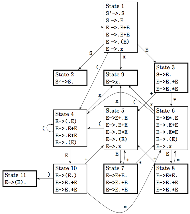
Let us carry this process out for our arithmetic expressions grammar, which we repeat here for convenience (with the added new state):
S' -> S
S -> E
E -> E + T | T
T -> T * F | F
F -> x | ( E )
To build the start state, we form the item set for the item S'->.S. For that, we need to look at production rules for S and add those in, as well as rules that start from the E that S gives rise to, and the T that the E gives rise to, and the F that the T gives rise to. So we have a lot of items:
S' -> .S
S  -> .E
E  -> .T
E  -> .E+T
T  -> .F
T  -> .T*F
F  -> .x
F  -> .(E)
All these together form one state in the DFA, the start state. We will number it as \(1\). This reflects all the possibilities when we are at the beginning of a “valid” string, on what we could expect next. We could expect an S if it has been formed, or an E or a T, or an F, or an x or an open parenthesis. These are all valid ways to start a string.
From state 1, we consider various possibilities for moving the marker. The simplest one is if we see an S. We find all items that have an S after the marker, and there’s only one such item. So we start an item set from S'-> S. and we would add other items if we had nonterminals to the right of the dot, but we don’t. So the second item set, numbered 2, would consist of only S'-> S., and we can transition to it from state 1. This is also an accept state, as it has an item in terminal form. There are no transitions out from that state.
We do the same for an input of E, resulting in the two items S->E. and E->E.+T. This is state 3, and it is also an accept state.
From state 3 we can transition on a “plus”, to a state that has the item E->E+.T as well as all initial items produced by P. This is state 4, and contains the following:
E -> E+.T
T -> .F
T -> .T*F
F -> .x
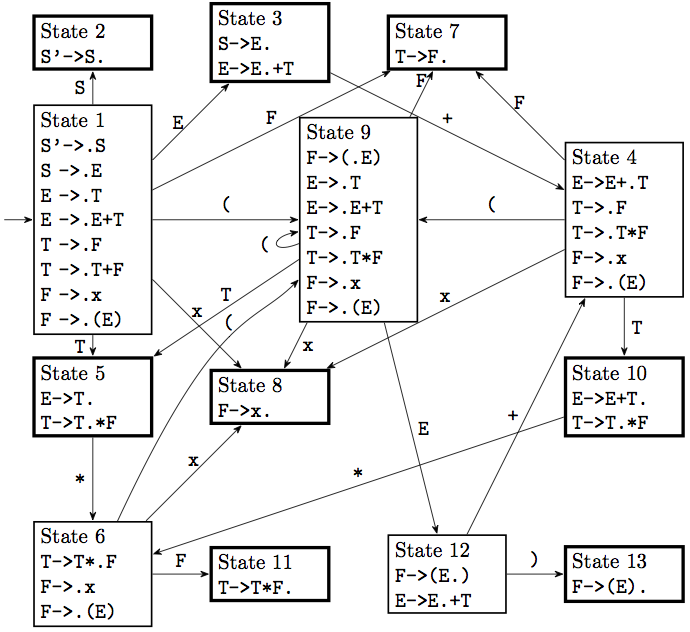
F -> .(E)We continue in this manner. Here is the resulting DFA:
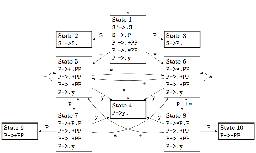
Exercise: As another example, here is the DFA for the polish notation grammar, do it yourselves before checking here:
Exercise (challenging): Understand the regular language that these DFAs recognize.
Now that we have seen this DFA generated by the item sets as described above, we will see how it relates to the LR parser.
Essentially the DFA keeps track of the progress that the parser is making towards productions, based on what is in its stack. It is convenient to add the state numbers in the stack to keep track of our progress. This way you can always look at the top of the stack and see what state you are in, and act accordingly.
Let us illustrate all this in the example of the string +*yyy in the polish notation. We start the PDA with the “empty stack symbol” in the stack, and in state 1, and we push the symbol 1 on the stack to remember this fact.
+*yyy $1 startNext our parser reads the input +, and pushes it onto the stack. At the same time it inspects that it is now in state 1, and follows the DFA from state 1 and on input + to arrive at state 5:
+*yyy    $1                 start
*yyy     $1+5               push +
Next we see read the input * and look at where the DFA would go from state 5 and on input *, and it goes to state 6:
+*yyy    $1                 start
*yyy     $1+5               push +
yyy      $1+5*6             push *
Next we read input y, push it and transition to state 4. These “moves” are called shifts, so we will start using the term.
+*yyy    $1                 start
*yyy     $1+5               shift +
yyy      $1+5*6             shift *
yy       $1+5*6y4           shift y
Now we are at state 4. There are no transitions from it, so we can’t “read” any more input. But luckily, this is an accept state, what we will call a reduce state: we have fully matched the rule P->y, so we need to dig into the stack, pop the y and add a P in its place. Before the y we were at state 6, so we now follow P from that state in the DFA to get to state 8.
+*yyy    $1                 start
*yyy     $1+5               shift +
yyy      $1+5*6             shift *
yy       $1+5*6y4           shift y
yy       $1+5*6P8           reduce 4
State 8 is not a reduce state, so we shift the next input, y, and transition to State 4. We then reduce it, put a P in the stack and transition to state 10 because of it:
+*yyy    $1                 start
*yyy     $1+5               shift +
yyy      $1+5*6             shift *
yy       $1+5*6y4           shift y
yy       $1+5*6P8           reduce 4
y        $1+5*6P8y4         shift y
y        $1+5*6P8P10        reduce 4
That is a reduce state, so we reduce it, using up the two Ps and the *, and going back to state 5, followed by pushing P on the stack and transitioning to state 7:
+*yyy    $1                 start
*yyy     $1+5               shift +
yyy      $1+5*6             shift *
yy       $1+5*6y4           shift y
yy       $1+5*6P8           reduce 4
y        $1+5*6P8y4         shift y
y        $1+5*6P8P10        reduce 4
y        $1+5P7             reduce 10
We now push our last symbol, y, onto the stack, shifting to state 4, then reduce that to get a P and transition to state 9, then reduce that to end up with a P from state 1, to state 3. That is followed by reducing \(P\) to \(S\) and making it to state 2, and at that point we can accept.
+*yyy    $1                 start
*yyy     $1+5               shift +
yyy      $1+5*6             shift *
yy       $1+5*6y4           shift y
yy       $1+5*6P8           reduce 4
y        $1+5*6P8y4         shift y
y        $1+5*6P8P10        reduce 4
y        $1+5P7             reduce 10
         $1+5P7y4           shift 7
         $1+5P7P9           reduce 4
         $1P3               reduce 9
         $1S2               reduce 3
As an illustration, we will carry out the same steps for the equivalent arithmetic expression x*x+x.
x*x+x       $1
*x+x        $1x8          shift x
*x+x        $1F7          reduce 8
*x+x        $1T5          reduce 7
Now we arrive at our first case of a problem. We have a reduce state, 5, but we could also shift from it. Which one should the parser do?
This is what we call a shift/reduce conflict. In some cases we can resolve these by looking at our follow sets, and doing a 1-token lookahead. The gist of it is that we should only reduce if we have a hope of continuing successfully, namely if the next input token is in the follow set of the nonterminal we are about to create with the reduction. In this case we would be creating an E, whose follow set consists of the terminals $, +, ). Since the next terminal is a *, we should not reduce, as we would be stuck (in other words, we are not ready for an E to be formed).
A true shift/reduce conflict exists only in the case where the next terminal is both a valid terminal for shifting and in the follow set for the corresponding reduction, leaving us with a hard choice to make. We will see an example later. In this case however, we proceed with shifting:
x*x+x       $1
*x+x        $1x8          shift x
*x+x        $1F7          reduce 8
*x+x        $1T5          reduce 7
x+x         $1T5*6        shift *
+x          $1T5*6x8      shift x
+x          $1T5*6F11     reduce 8
+x          $1T5          reduce 11
Now we are in the same predicament, at state 5, but now the lookahead symbol is a +, in the follow set. It is also not a symbol that we can shift. We therefore will reduce:
x*x+x       $1
*x+x        $1x8          shift x
*x+x        $1F7          reduce 8
*x+x        $1T5          reduce 7
x+x         $1T5*6        shift *
+x          $1T5*6x8      shift x
+x          $1T5*6F11     reduce 8
+x          $1T5          reduce 11
+x          $1E3          reduce 5
Now we are presented with a similar problem on state 3. We can reduce to S, or we can shift on a +. Since + is not in the follow set of S, there is no conflict and we proceed by shifting.
x*x+x       $1
*x+x        $1x8          shift x
*x+x        $1F7          reduce 8
*x+x        $1T5          reduce 7
x+x         $1T5*6        shift *
+x          $1T5*6x8      shift x
+x          $1T5*6F11     reduce 8
+x          $1T5          reduce 11
+x          $1E3          reduce 5
x           $1E3+4        shift +
            $1E3+4x8      shift x
            $1E3+4F7      reduce 8
            $1E3+4T10     reduce 7
Another possibility for shift/reduce conflict. The shifting makes sense on a *, the reduction makes sense on the follow set of E, which luckily does not contain *. In our case the lookahead is $ (end of input), so we want to reduce. We then land back at our state 3 conflict, which we now reduce because of the lookahead. This lands us on state 2, our accept state. And this completes the computation.
x*x+x       $1
*x+x        $1x8          shift x
*x+x        $1F7          reduce 8
*x+x        $1T5          reduce 7
x+x         $1T5*6        shift *
+x          $1T5*6x8      shift x
+x          $1T5*6F11     reduce 8
+x          $1T5          reduce 11
+x          $1E3          reduce 5
x           $1E3+4        shift +
            $1E3+4x8      shift x
            $1E3+4F7      reduce 8
            $1E3+4T10     reduce 7
            $1E3          reduce 10
$1S2 reduce 3When we construct the table of transitions for the DFA for a grammar, there are a couple of conflicts that can occur:
Let us see these conflicts in action. Suppose we attempt a simplified arithmetic expression language, that tries to do away with the T and F nonterminals:
S -> E
E -> E + E | E * E | (E) | x
We start by computing first and follow sets. Do this first on your own:
Nonterminal        First set          Follow set
-----------        -----------        -----------
S                  x, (               $
E                  x, (               ), *, +, $
Here is the DFA of the item sets:
Let us consider all the conflicts present, starting with state 3. On state 3 we don’t have a shift-reduce conflict, since the final set of S, namely $, does not conflict with the shift options.
State 7 has some true conflicts. First, on input symbol + it has a shift/reduce conflict. It can either choose to reduce the term E+E it has seen so far into an E, or else it can shift to the plus, ending with E+E+ on the stack, and planning to match the second E with another E later on. Essentially this is the question of associativity of the operator. Choosing to reduce makes the operator left-associative, choosing to shift makes the operator right-associative. Most parser generators allow us to specify this choice, rather than requiring us to rewrite the grammar.
State 7 also has a conflict on input *. In this case it has the choice of first doing the addition, and doing a multiplication further down, or going for the multiplication first. This is a question of precedence of operators; shifting indicates that multiplication takes precedence, reducing means addition takes precedence. On state 8 and input + these roles are reversed. Again, most parser generators will allow you to specify precedence of tokens, and will use that precedence to automatically resolve such conflicts.
Exercise: Consider the grammar:
S -> A|B
A -> xA|eps
B -> xBy|eps
Compute the first and follow sets, and the DFA for LR-parsers of this grammar, and show determine any conflicts that are present, and the reason for their presence.
Exercise: Do the same for the following grammar for conditional expressions. We use angle brackets here to denote the nonterminals, as our terminals are whole words:
<start> ::= <boolexp>
<boolexp> ::= TRUE | FALSE
            | IF <boolexp> THEN <boolexp>
            | IF <boolexp> THEN <boolexp> ELSE <boolexp>