Prediction error. Constant model
In modeling our goal is typically to explain and/or predict the values of a target variable, given values of other variables and some modeling assumptions.
Here are some key terms:
A specific formula / function of the predictor variables and some parameters, whose output is meant to model the target variable. We would write this in general form as:
\[Y \sim f(X_1, X_2, ...; \beta_1,\beta_2, ...)\]
where \(Y\) is the target variable, \(X_1\), \(X_2\), … are the predictor variables, and \(\beta_1\), \(\beta_2\), … are parameters, values to be determined.
The “Sum of Squared Residuals”, sometimes called “Residual Sum of Squares”. This is a measure of the overall error you are making at all your data points together.
Some times we adjust this by dividing by \(n-1\) or something similar.
Normal modeling techniques try to choose the parameters so as to minimize this sum.
It is important to identify some key steps in the process:
We will focus exclusively on linear functions of one predictor variable, so we will not be able to do many of these. But in this introduction I will talk about some of these concepts in more general terms.
Here are some basic examples of the above ideas. Our target variable is student GPA, we want to try to find a way to predict it.
This is the simplest model we can try to fit. We have no predictor variables, so all we can do is predict a single number: \[Y \sim \beta\] Where \(\beta\) is the parameter. All we have to do to “fit” the model is to provide a constant value for the parameter. So we could for instance say \(Y \sim 2.93\), meaning that we predict that the student’s GPA is equal to \(2.93\).
The predicted values in this case are always equal to this constant value. The residuals are the differences \(y - \beta\).
It turns out, that if we want to choose a value for \(\beta\) that makes the SSR as small as possible, then we must choose \(\beta = \bar y\), the mean of the \(y\) values.
The best constant model fit is when that constant is equal to the mean of the \(y\) values, \(\bar y\). The Adjusted SSR measure in this case equals the variance of \(y\).
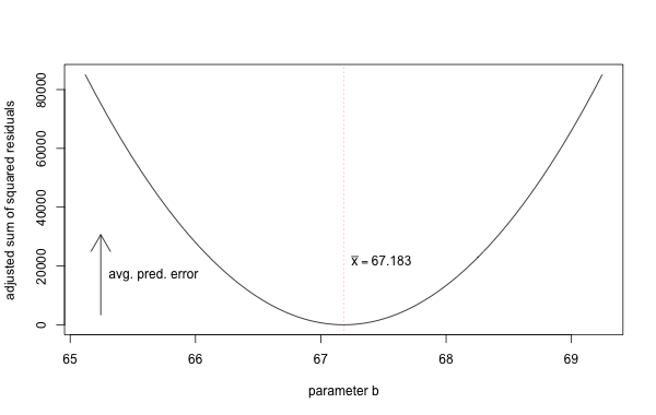
As one example of this, consider the behavioral survey data we have been looking at. If we were asked to fit a constant model to the height variable in that dataset, then we would make the model \(Y\sim 67.183\) as that value is the mean. We can see that this value is the one that minimizes the “sum of squared residuals”: \[\frac{\sum(y-\hat y)^2}{n-1}\] In the case of a constant model, that ends up being what we called the variance, because \(\hat y\) is always equal to the mean \(\bar y\).
If we try to compute the sum \[\frac{\sum(y-b)^2}{n-1}\] for different values of \(b\), we can see that the mean achieves the smallest value. In the following graph, the \(x\) axis represents possible values for the constant \(b\), and the \(y\) axis represents the corresponding average squared prediction error for that constant. Our goal is to minimize that error.

Prediction error. Constant model
Another common case is when we try to have a predictor variable that is categorical. These are often called “factors”. For instance we could say that we will try to predict the student’s GPA based on their gender.
In this case we would basically need to provide two parameter values: One parameter for our guess for the GPA if the student is male, and another for the GPA if the student is female.
It turns out that the best guesses in this case are again the means of the male and female students respectively:
The best model for the case where \(Y\) is a scalar variable and \(X\) is a categorical variable is to assign for a particular value \(x_0\) the average of the \(y\) values for those cases whose \(x\) value equals \(x_0\).
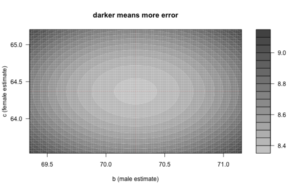
As an example, in the behavioral survey, one of the variables is the gender. To build a model that based on the gender tries to predict the height, we simply need to provide a value for the male gender, and a value for the female gender. These values are respectively the height averages for males and females, \(70.252\) and \(64.368\) respectively.
In this case our model \(Y\sim f(X)\) has two parameters: \(f(\textrm{male}) = b\) and \(f(\textrm{female}) = c\). These are chosen so at to make the corresponding sum of squared residuals as small as possible. The following two-dimensional graph gives us a sense of where this minimum overall error is achieved. The darker areas correspond to more error.

Prediction error. Factor model
The most common model, and one we will spend more time with next week, is that of a linear equation. For example, perhaps we think that a student’s high-school gpa should be a good predictor of their college gpa. In that case, if we denote a student’s high-school GPA with \(x\) and their college gpa with \(y\), we would be looking for an equation of the form:
\[y = \alpha + \beta x\]
Where \(\alpha,\beta\) are the parameters, and we would like to choose their “best values” to fit the data in any given scenario. We will explore this more in the next section.