A regression line
Sections 7.1-7.3
When the data appears to have an overall linear direction, it would be reasonable to attempt to obtain a linear model fit, so an equation of the form:
\[y \sim a + b x\]
where \(a\), \(b\) are the two parameters to be determined.
Notice that unlike what you may be used to, we use \(b\) to denote the slope of the line, and \(a\) to denote the \(y\) intercept.
The least squares regression line is the linear equation with the smallest sum of squared residuals (SSR).
It is obtained by computing \(a\), \(b\) according to the formula:
\[b = r\frac{s_y}{s_x}\]
\[a = \bar y - b \bar x\]
Let us see this in action in the example of the city mileage and the highway mileage:

A regression line
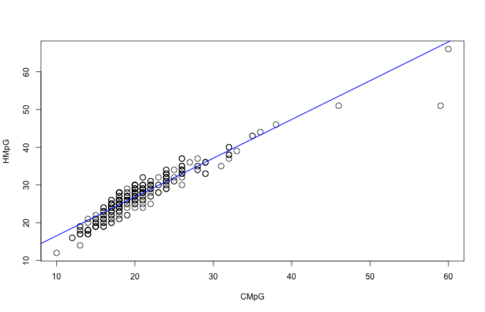
There is overall a linear direction, and therefore it makes sense to look for a linear equation like that. Let’s see how we would compute the equation for that line by hand. We will need to know the means and standard deviations for both CMpG (our x variable) and HMpG (our y variable):
| Variable | Mean | Std. Dev | Correlation |
|---|---|---|---|
| CMpG HMpG | 20.09 26.90 | 5.213 5.967 | 0.94 |
It is really important to not forget which variable is your \(x\) and which is your \(y\), or you’ll get the formulas all wrong. In our case, CMpG is our \(x\).
So let us compute the regression line. Slope first:
\[b = r \frac{s_y}{s_x} = 0.94\times \frac{5.967}{5.213} = 1.076\]
\[a = \bar y - b \bar x = 26.9 - 1.076\times 20.09 = 5.283\]
So our final equation for the regression line is:
\[\hat y = 5.283 + 1.076 \times x\]
We used \(\hat y\) there instead of \(y\) because that equation gives us the predicted values, not the actual \(y\) values in the data.
Let’s use this line to do some prediction. For instance, suppose we have a car that has CMpG of 20. We would then predict that its HMpG would be:
\[5.283 + 1.076 \times 20 = 26.803\]
so we would predict a highway mileage of \(26.8\) for such a car. Now if you look at the graph, you will see that there a number of cars with CMpG of 20, whose corresponding HMpGs range from around 24 to 30. There is no way for our model to predict all those accurately: Our model can only make one prediction from the CMpG of 20. So it’s bound to make some errors. But it’s doing as best as we could expect it to.
There is a certain interpretation afforded to the square of the correlation, \(r^2\). In order to understand it, we have to understand the main goal of modeling.
When we use a linear equation \(y=a+bx\) as a model, we are in effect saying: “We know \(y\) is changing, and we believe it is because \(x\) is changing, and this formula tells us about this change.”
We can think of that equation as “explaining part of the variance in \(y\)”. It does it via the predicted values \(\hat y\). Since \(\hat y\) is exactly equal to \(a+bx\), all the variation that \(\hat y\) undergoes is directly caused by the corresponding variation in \(x\). This is where \(r^2\) comes in:
\[r^2 = \frac{\textrm{Variance}(\hat y)}{\textrm{Variance}(y)}\]
\(r^2\) measures the percent of the variance of \(y\) that is explained by the variance in \(x\).
In our example, \(r=0.94\) and so \(r^2=0.8836\). So we can say that 88% of the variation we observe in HMpG can be explained by the corresponding variation in $CMpG.
In fact something further happens: The overall Variance is decomposed in two parts:
\[\textrm{Variance}(y) = \textrm{Variance}(\hat y) + \textrm{adjusted SSR}\]
Quite literally, the overall variance is a sum of the variance of the predicted values, plus the adjusted square error, which we can think of as the leftover variance that we have not yet explained via the linear relation.
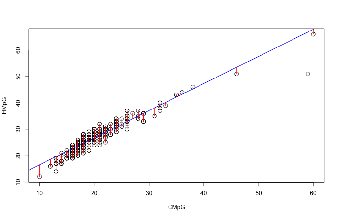
Recall that the residual is the difference between the \(y\) value and the corresponding \(\hat y\) predicted value. Geometrically we can think of the residuals as the vertical distances from each point to the regression line:

The residuals
Think of the residuals as springs attached to the line. The further they are, the more stretched out the springs, and the stronger they pull the line towards them:
The goal of the least squares regression line is to be as close as it can to its points, resulting in small residuals.
The line will try to move towards points with large residuals, if it can do so without sacrificing too much on the other points.
Here is a little applet to play with to investigate the effect of residuals on a page:
There are two kinds of outliers:
Outliers that are far in the \(x\) direction (possibly also the \(y\) direction) will affect both the slope and the intercept of the line (line changes slope to move towards them).
Outliers that are far only in the \(y\) direction will not affect the slope much, but will affect the intercept (line moves parallel up or down towards them).
Outliers that affect the slope are usually called influential.
In a residual plot, we draw a graph of the residuals on the \(y\) axis, against either the \(x\) or the predicted \(\hat y\) values, or occationally against other variable’s values.
The effect of this is that it accenuates any non-linear patterns that were possibly not visible because of the dominance of the linear effect.
In a residual plot, we look for the absence of a pattern. Since the residuals are the error our model makes when predicting values, they should appear to be just random “noise” if our model accurately captures the interaction between the variables.
If a pattern exists in the residual plot, it is an indication that our model does not accurately capture the behavior of the data, that there is something else going on.
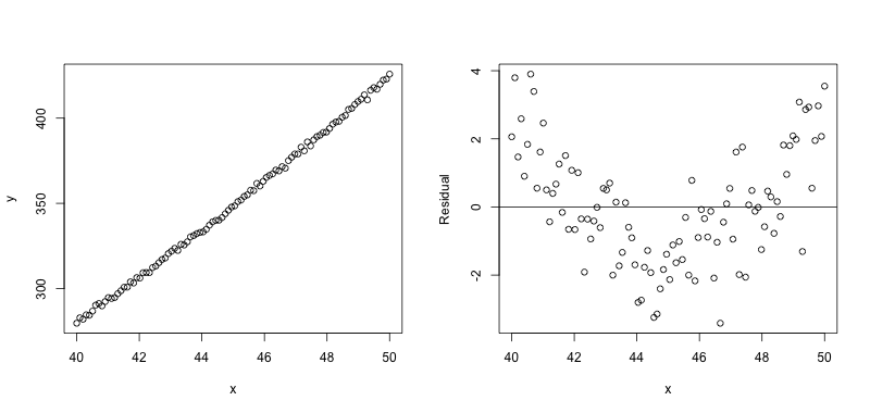
Here is an example of such a situation. The data does look extremely linear, and a linear model would be a good fit. In fact the correlation coefficient is \(r=0.9992\), indicating an extremely strong linear relation. The residual plot on the right however, shows that the residuals have a distinct curve to them. This is because the data actually follows a slightly quadratic pattern, that we cannot see because it is imperceptible. When we take the linear part out of the picture, the need for the quadratic term becomes clear.

Residual plot
Studying these models goes beyond the introductory nature of this course.