Tree Diagrams

Reading

Sections 2.2.6, 2.2.7

Practice Problems

2.6.2 (Page 119): 2.22, 2.23, 2.24, 2.25, 2.26

Notes

Tree Diagrams are a way to visualize random processes with multiple steps. They help us keep track of what is what along the way. Here are the main components:

Root

There is a root of the tree, which is considered our starting point.

Branch Levels

Each branching level from that point on corresponds to one step in the process. For instance when rolling a die 3 times, there will be three steps corresponding to each of the 3 rolls.

At each branching level there is a number of different paths to follow, corresponding to mutually exclusive events that exhaust all possibilities. Each path taken amounts to selecting a particular event to occur.

For example in the event of rolling a die three times, and if we only cared about whether each outcome is even or odd, we would have two paths at each branching point, corresponding to those two possibilities.

Leaves

Each “full path” through the tree, ending in a leaf, corresponds to one outcome of the whole process, that outcome being the intersection of all the events along the path.

Branch probabilities

At each branch point, each branch from that point has a corresponding conditional probability of taking that branch, given that we are already at that point.

The probabilities for all branches from a given branch point must add up to 100%.

Leaf probabilities

At each leaf, as well as each branch point in the tree, there is a corresponding probability of making it to that point starting from the root.

To find this probability, multiply the probabilities of all the branches taken to get there.

An example

An illustration will help. Consider the following problem:

Two teams A and B will play in a “best out of 3” series of games. On any particular game, team A has a 60% chance to win, while B has only a 40% chance.

What are the overall chances that team A will win?

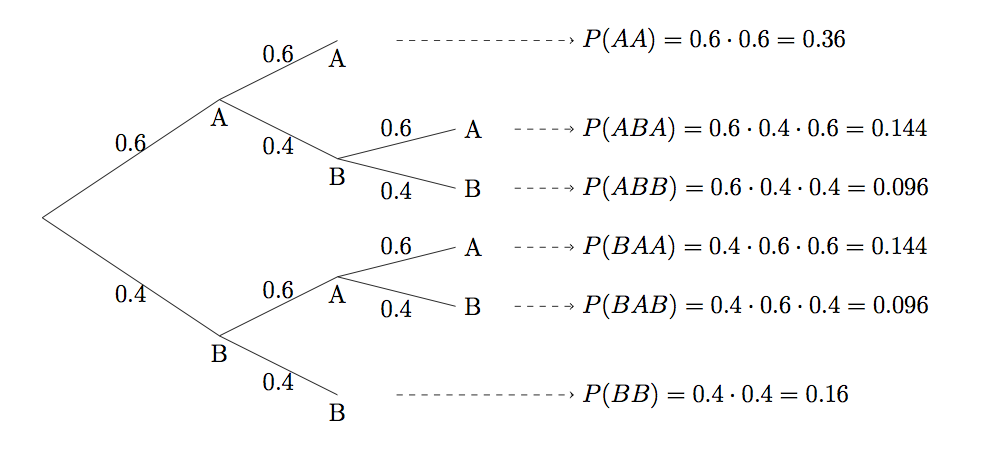
Here is how a diagram for this problem might look like.

Tree Diagram, “Best out of 3”

You can see that we have one branching point for each game, with two options each time depending on which game wins. The conditional probabilities along the branches are always \(0.6\) and \(0.4\).

Notice that some paths only need to go 2 levels deep, as a third game is not always necessary.

So now to find the overall chances of team A winning, we have to follow all the paths that end up with a win for A. These are the paths AA, ABA and BAA. They are disjoint, so we add their probabilities:

\[P(AA) + P(ABA) + P(BAA) = 0.36 + 0.144 + 0.144 = 0.648\]

So team A has a \(64.8\)% chance of winning a “best out of 3” against team B. Their chances went up vs a single game: This is because the more games they have to play, the more opportunities they have to assert their 60% superiority.

As a better illustration of that, imagine they played 500 games. How likely are they to win over half of those games? The more they play, the more pronounced the difference between 40% and 60% becomes.

We will now consider a number of related questions:

If team A does end up winning, what are the chances that a third game was necessary?

Overall, what are the chances that a third game is necessary?

If a third game was necessary, what are the chances that team A won?

If only two games were needed, what are the chances that team A won?

Let us try to answer those questions.

The first is simple. It is a conditional probability, given that team A ended up winning. So it will be a quotient, where the denominator is all the ways team A wins an the numerator are those ways in which team A wins and 3 games are played. So we would have:

\[\frac{P(ABA) + P(BAA)}{P(AA) + P(ABA) + P(BAA)} = \frac{0.288}{0.648} = 0.4444\]
So the chances that a third game was necessary given that A won are \(44.44\)%
Now we proceed to the second question, the chances that a third game was necessary. To do that, we actually want to stop earlier in the paths. So we want to follow the two middle paths, AB and BA, but only up to that point, as those are the two locations that would necessitate a third game. The chances would therefore be:

\[P(AB) + P(BA) = 0.24 + 0.24 = 0.48\]

or 48%. Another way to do the same problem would have been to look at the complement, which would have been that the series ended in 2 games, then subtract that probability from 1. This would be:
\[1 - P(AA) - P(BB) = 1-0.36-0.16 = 1-0.52=0.48\]
For the third question, it is again a conditional. We need to compute a quotient where the denominator is what we just computed, and the numerator is those paths with 3 games that ended up in a team A win. So we would have:

\[\frac{P(ABA) + P(BAA)}{0.48} = \frac{0.288}{0.48} = 0.6\]

So the chances are 60%.
Take a moment to ponder this: The chances of A winning, given that we know a third game was necessary, are the same as the chances of A winning a single game. There is a very simple explanation for that, make sure you figure it out.
This is similar to previous problems. The computation would be:

\[\frac{P(AA)}{P(AA) + P(BB)} = \frac{0.36}{0.52} = 0.6923\]

So there is a \(69.23\)% probability.

Medical tests

Tree diagrams and conditional probabilities can help us understand the setup on most medical tests. There are two key components: The sample and the test. This is more generally the setup for what is known as “binary classification test”.

We want to test if a particular person has a particular disease. Whether the person has the disease or not is the sample, and it can be positive or negative.

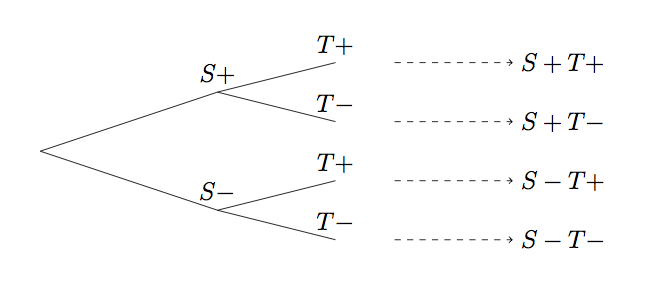
Then we perform the test. The test can come out positive or negative as well. So we have in total 4 cases:

Positive sample, positive test (S+T+). This is a correct diagnosis.
Positive sample, negative test (S+T-). This is a false diagnosis, and is known as a false negative. This is a severe case, as the person has something and we told them they are fine.
Negative sample, positive test (S-T+). This is another false diagnosis, known as a false positive. This is less severe in a way. We are probably unnecessarily alarming the person, but followup tests should clear things up.
Negative sample, negative test (S-T-). This is another correct diagnosis.

We can represent this as a 2-step tree diagram: The first step is whether the sample is positive or negative, the second is whether the test is positive or negative.

Tree Diagram, medical tests

The probabilities associated with the first branches are \(P(S-)\) and \(P(S+)\). These are the chances that the person is positive/negative, so for these we need to know some population statistics, i.e. what percent of those who go for a test are positive/negative.

The second set of branches is more interesting. It contains things like \(P(T-|S-)\), i.e. conditional probabilities, given that we know if the sample is positive/negative, of getting the test to be positive/negative. These are usually known to us by the work that was done during the development of the test: The test was probably tested on a number of samples that we knew were positive/negative, and we measured how many times it was right/wrong. These probabilities have specific names:

sensitivity: This is \(P(T+|S+)\), in other words the percent of positive samples that are correctly classified. Also known as true positive rate or recall rate.
false negative rate: This is \(P(T-|S+)\), i.e. the percent of the positive samples that are misclassified. This is complementary to the sensitivity.
specificity: This is \(P(T-|S-)\), i.e. the percent of negative samples that are correctly classified. It is also known as true negative rate.
false positive rate: This is \(P(T+|S-)\), i.e. the percent of negative samples that are misclassified. Complementary to the specificity.

Both sensitivity and specificity are important: Sensitivity is the test’s ability to detect positive patients, specificity is its ability to detect negative patients.

Let us work out a specific example. Suppose we try to diagnose a disease that only 5% of the population has (so \(P(S+) = 0.05\) assuming all people are equally likely to come in for a test). The particular test we will employ has a specificity of \(0.96\) and a sensitivity of \(0.99\). In other words, it misclassifies one in every 100 positive samples and 4 in every 100 negative samples.

The question of interest in practice is this: If the test comes out negative, what are the chances that the person is in fact negative?

This is in fact a conditional probability given a test result, which is the opposite of what we are given as part of our inputs.

In binary classification tests / medical diagnosis we know \(P(T\pm|S\pm)\) and we need to find out \((S\pm|T\pm)\).

For instance let us compute \(P(S-|T-)\):

\[P(S-|T-) = \frac{P(S-T-)}{P(T-)} = \frac{P(S-T-)}{P(S-T-) + P(S+T-)}\]

We can use the tree diagram to compute the required probabilities:

\[P(S-T-) = P(S-)P(T-|S-) = 0.95 \cdot 0.96 = 0.912\]

\[P(S+T-) = P(S+)P(T-|S+) = 0.05 \cdot 0.01 = 0.0005\]

So we can now finish the computation:

\[P(S-|T-) = \frac{0.912}{0.9125} = 0.99945\]

So this is nice, if the test is negative we have a very high probability of being negative, and a very small (\(0.00055 = 0.055\%\)) of being positive.

For practice:

Work out the chances of being positive given that the test came out positive.
Work out the same questions if \(P(S+) = 0.4\), i.e. if we had more of the positive people coming in for tests, and not as many of the negative people.